Stocks and Bonds

Stocks and bonds are often combined to create more balanced portfolios. Since stocks and bonds are often negatively coorelated, poor performance in stocks can partially be set off by bonds and vise versa. In this project we will quantify this effect and analyze the tradeoff between stocks and bonds.

Historical Data

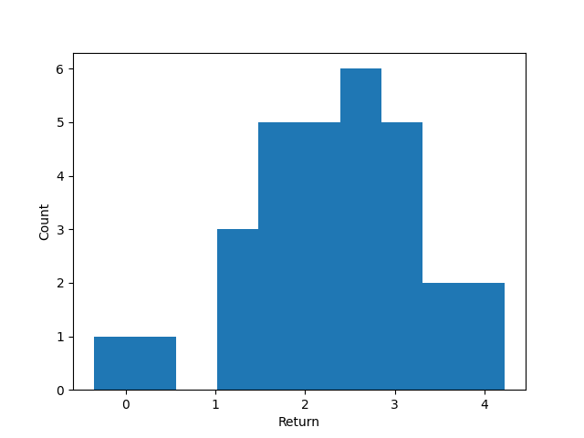
In this project we fit historical data of stocks, bonds, and inflation from macrotrends and FRED going from 1990 to 2020. The stock and inflation data is visualized in my previous post. Here we plot the bond data to ensure it makes sense.

We fit a normal distribution to the returns.

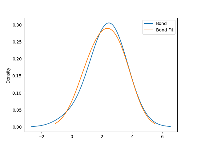
For stocks, bonds, and inflation we have a mean of 9.87, 2.31, and 4.25 respectively. Inflation used to be much higher and outside of recent inflation has consistently been around 2% (the FED's target). Therefore, we will use the 2% figure going forward.

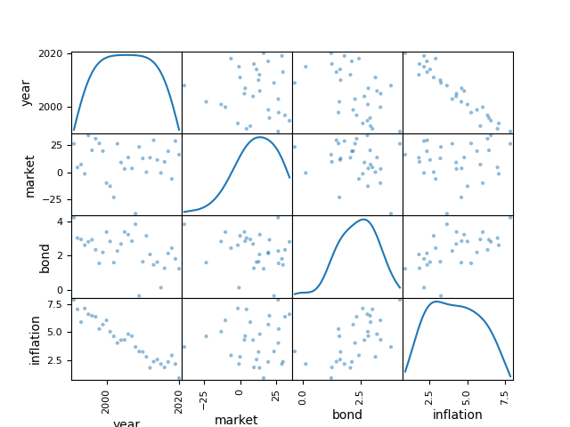
As mentioned before, the coorelation between stocks and bonds is important to create a successful portfolio. A scatter matrix is always a good start.

To obtain a quantitative estimate we calculate the coorelation matrix between our variables.

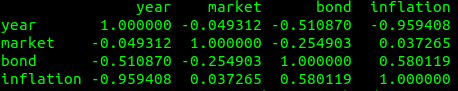
We can see that market with bonds and bonds with inflation have a reasonable coorelation. This will be important when building our model.

Simulation

Using the computed means and coorelation matrix from the previous section, we draw from a multivariate normal using numpy. After the samples are drawn and structured in the same manner as my previous post, let the stock allocation $0 \leq r \leq 1$ and the return is
$$\text{TR} = (r\text{SR}+(1-r)\text{BR})/\text{I} .$$

With a 60% stock allocation we recieve a distribution of returns that looks like this after 30 years.

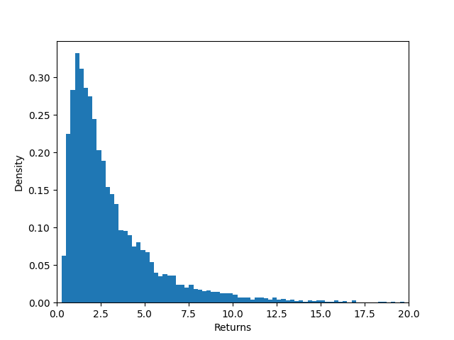
Much like the last time, it is a right skewed distribution with a median of 4.39 and a standard deviation of 5.62.

Sharpe Ratio

We want to know what happens when we change the stock bond allocation. To quantify this we simulate many different stock bond allocations to show return against allocation and volatility against allocation.

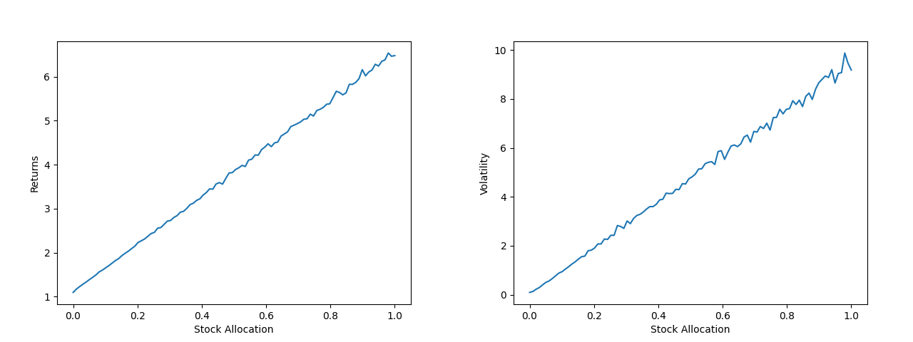
We see that median returns increases as stock allocation increases as expected. However, it comes with a penalty of increased volatility. To get an idea of how much return is earned for a unit of volatility we use the Sharpe ratio with the risk free return being the portfolio with 0% stocks.

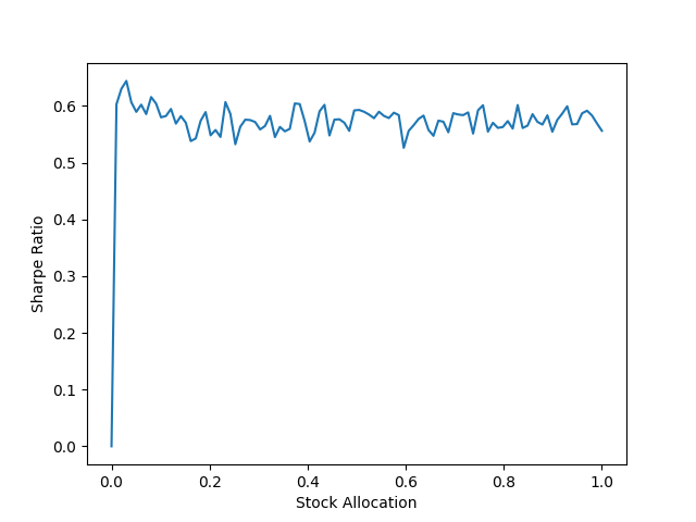
The Sharpe ratio is between 50-60%. To increase this ratio we would want to add higher yield and uncoorelated assets.

Conclusion

Using the Monte Carlo method we simulated a mixed portfolio of stocks and long-term government bonds. Bonds act as a great stabalizing factor in a portfolio. Stocks offer much greater returns at the cost of higher risk. When building a portfolio for savings or retirement a balance should be struck between the two.

Lastly, this analysis ignores some things for simplicity. For example, one could combine stocks, government bonds, and corporate bonds. Model the distributions with non-normal distributions using a copula. The later is very important when accuracy is important. This is because tail risks and black swan events can have a massive impact over longer time spans. This project is just a starting point. My code can be found here. Have fun!