Outline

Analysis of the stock market can be an incredibly complex subject. Markets go up and down, the country goes through recessions, our gains are subject to inflation, and so much more. It seems too complex to model exactly, but it would be nice if we could get an idea of what our returns would be.

In order to avoid the complexities of modeling every interaction possible we instead use probability and statistics to develop a distribution of possible stock and bond yields and inflation rates and simulate a large number of possible market conditions until we form a distribution of returns. This strategy of simulating a large number of possible outcomes is called the Monte Carlo Method and used very often in physics and mathematics.

Historical Data

It is often said that history repeats itself, and for modeling the stock market it is not a bad start. For this project we will be using inflation data from FRED that has data from 1960-2020 and the returns of the S&P 500 from macrotrends with data from 1928-2022. We start by plotting the historical data.

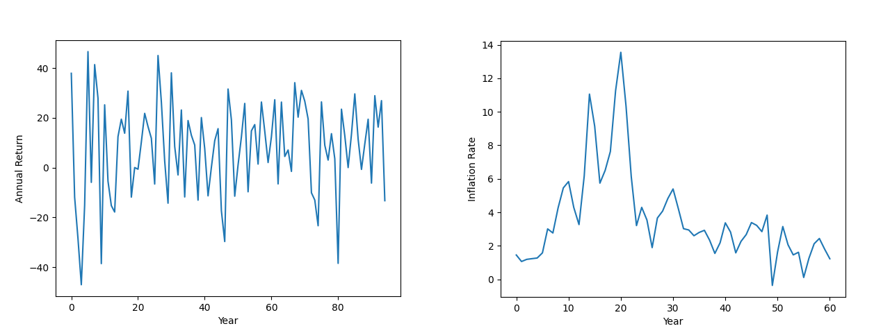
The historical data looks very complicated. It has stochastic ups and downs with no clear pattern. Things will look clearer when we plot the historical distribution of returns and inflation.

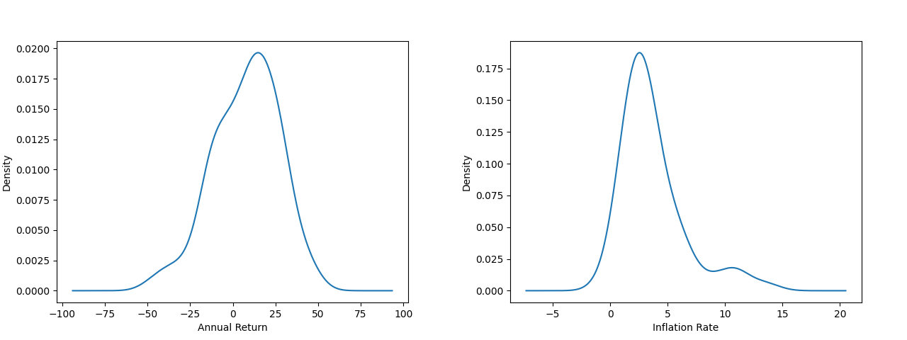
Neither of these distributions is a standard distribution like the normal, but it will be very useful to fit a slanted normal to the stock data and a normal to the inflation data. The slanted normal is a good assumption for the stocks because the S&P 500 is made up of well-performing companies and would not be in the index if they performed poorly on average. We use the last 30 years of data (orange) and have the following fits (blue).

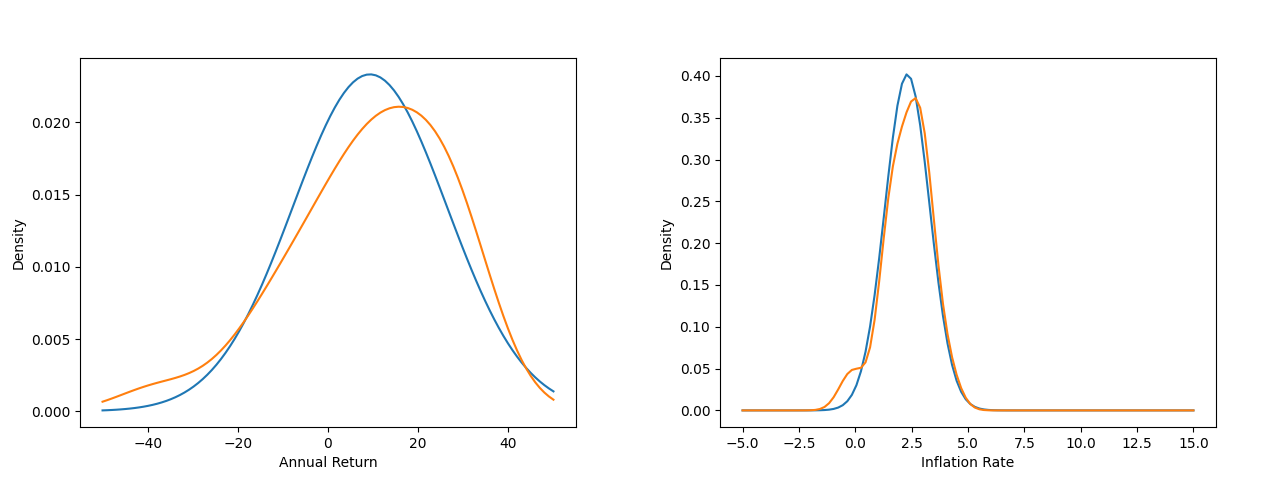
For the stocks we have a return mean of 9.3% with STD dev 4.1% and for the inflation we have a mean rate of 2.3% with STD dev 1.0%. Although it is not a perfect fit, we are sacrificing accuracy for a more interpretable model. For example, with this model we can easily modify parameters like the mean, shape, and standard deviation to model more adverse market conditions. If we had simply used a black box by constructing the density of the historical data we would not have this luxery. Now we are ready to perform the simulation.

Simulation

Let $n$ be the number of years we wish to simulate and $m$ the number of simulations to run. We construct a matrix of returns $R$ and inflation rates $I$ of size $n \times m$. Converting them to percentages and adding $1$, the total return on each simulation $s_i$ is the initial amount multiplied by the product of all elements in the in the $i$-th column of $R$. The same process is done to the matrix $I$ and taking the reciprocal. Multiply the two results for each simulation to get the final answer. Letting $\Pi_i A$ denote the product of all elements in the $i$-th column our formula for $s_i$ is
$$s_i = A_0\left(\Pi_i (1+R) \cdot 1/\Pi_i (1+I) \right) .$$
These operations are vectorized in numpy and runs very quickly. The time complexity is $O(mn)$. As we generally fix the number of years $m$ (or at the very least is bounded), it behaves like a constant the time complexity is more akin to $O(n)$, which is incredibly fast.

We are now ready to plot the return of distributions. Let $A_0=1$ and we have the following plot.

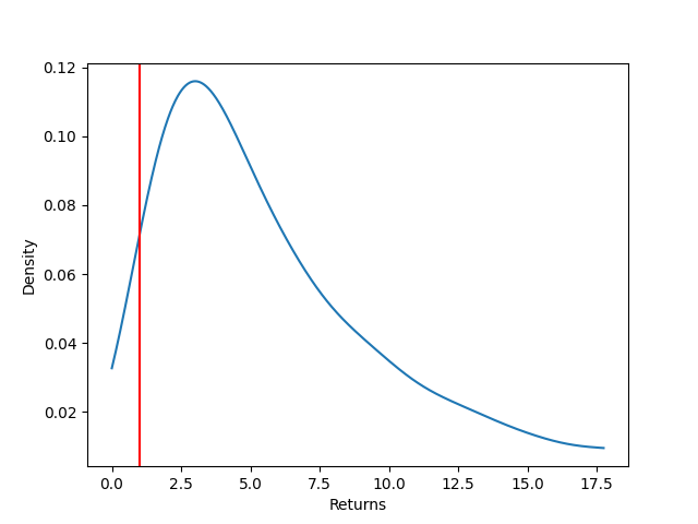
We can see that sometimes we end up losing money but happens rarely. Calculating the moments gives us a better idea than the picture. We end up with a mean, standard deviation, and skew of 7.34, 7.73, and 3.49. This shows that we are expected to make a $7.34$ times on our investment. The standard deviation tells us that the returns are not very well centered (it is large in comparision to the mean). The positive skew then tells us that a lot of the mass is on the left side of the mean (which is unfortunate). In fact, running the simulation several times gives that approximately $62.84 \pm 0.15 \%$ of the distribution lies to the left of the mean. This analysis lets us say that we are expected to make $7.34$ times on our investment, and although we can do better, we ore often do worse. The advantage of doing more simulations is that we can better picture the distribution of returns and give confidence intervals to our statistics. Although it sounds worrying that we have a right skewed distribution, adding other assets like bonds can help stabalize the fluctuations in the stocks.

Conclusion

Although this is a simple model with historical data, there are many things that can be added quite easily to this simulation. One can add new asset classes like bonds and analyze how stock-bond allocation impacts the return distribution. Another useful addition would be to pull a certain amount every year like a retirement acount. Changing shape parameters on our distributions can give us more intution on how much an impact each one has on our returns. To experiment with your own designs you can clone the repository at my Github. Enjoy!