Mexico City Metro

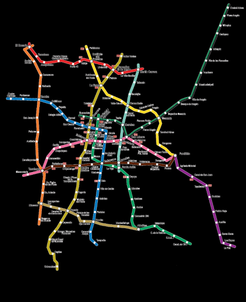
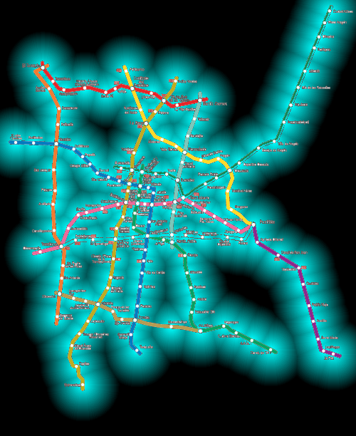
Mexico City has one of the largest metro systems in North America. Using the metro, one can go just about anywhere in the city for five pesos. It is a truly massive system with 195 stations. In this project we wish to calculate the distance (as the crow flies) to the nearest metro station at any point in the city. Downloading the metro map from the government website and changing the background to black gives.

Locating Stations

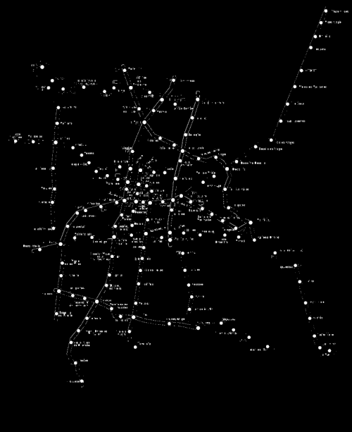
The hardest part of this project is actually locating the stations. Looking at the metro map we see that the metro stations are marked by large white dots. However, the main problem we face is that the station names are also written in white. This is a big problem as there are other sources of white other than the stations in the image. As a preprocessing step, we first turn all the pixels that are not close to white black.

Next we parse the processed image looking for blobs. We define a blob as a contiguous block of white pixels. Whenever a white pixel is found we perform a breadth first search to find all pixels in the blob. Blobs that do not contain enough pixels are turned black. Because each pixel is only processed once the algorithm runs in $O(nm)$ time where $n$ and $m$ are the length and width of the image respectively. When this algorithm is performed we obtain the following.

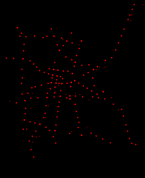
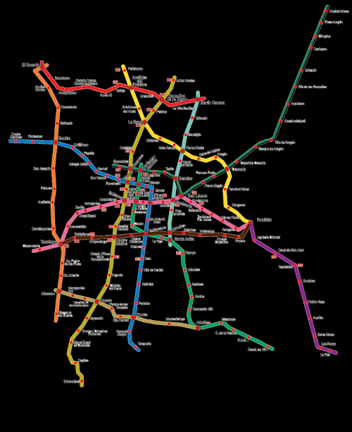
This is pretty good! We can see that there are some miscellaneous blobs left over. We fix this by just going over the image directly in GIMP. We then perform the same exact algorithm again with the cleaned file. Overlaying it with the original metro map we see that we get all the stations.

Calculating Distance

To calculate the distance to the closest metro station at every pixel we go pixel by pixel and calculate the minimum distance of all the metro stations. This runs in $O(nmV)$ time where $n$, $m$, and $V$ are the length and width of the image and $V$ is the number of stations. Reducing the complexity would likely require taking into account the connectivity of the metro which would be much more difficult. Therefore, I simply scaled the map where $n, m \sim 500$. This allows the algorithm to run in a decent time and still yields accurate results. Color coding based on distance gives the following aesthetic image.

Conclusion

I am actually really pleased with the result obtained, but there are always ways in which it could be improved. I think the major one is in the distance calculation. If the stations were connected via a graph data structure I believe there would be a way to reduce the complexity. Heuristically, given the closest station of a neighboring pixel, the current pixel's closest station should not be too far. There are of course exceptions but it is a good heuristic to search with.

However, the main advantage to connecting the stations in a graph is that one could then calculate trip times. Given a walking rate and the metro times, one can get a rough arrival time by adding the time it takes to get to the station, traverse the metro, and then walk to the destination. Although I did not do it for this project, perhaps the most efficient way to do it would be to connect every station to all data points within a certain radius. It will not be perfect, but it will hopefully be good enough that it requires minimal editing. For those curious, the algorithm falls under the method of persistent homology.

As always, my code is linked. Enjoy!